
See the Actflow Toolbox for more information
Run the code yourself here: https://github.com/ColeLab/ActflowToolbox/blob/master/examples/HCP_example.ipynb
#Import packages and set variables
import numpy as np
import h5py
import pkg_resources
import matplotlib as mpl
import matplotlib.pyplot as plt
import seaborn as sns
from scipy import stats
import sys
sys.path.insert(0, '../../')
#Used for plotting brain images inline
from wbplot import pscalar
import matplotlib.image as mpimg
%matplotlib inline
plt.rcParams['image.interpolation'] = 'none'
plt.rcParams['figure.figsize'] = 6,4
plt.rcParams.update({'font.size': 16})
plt.rcParams['image.aspect'] = 'equal'
plt.rcParams['image.cmap'] = 'seismic'
import ActflowToolbox as actflow
actflow_example_dir = pkg_resources.resource_filename('ActflowToolbox.examples', 'HCP_example_data/')
networkpartition_dir = pkg_resources.resource_filename('ActflowToolbox.dependencies', 'ColeAnticevicNetPartition/')
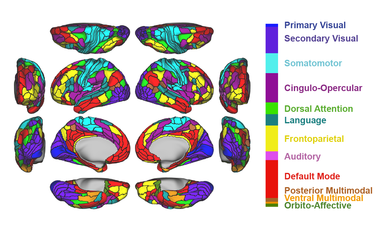
networkdef = np.loadtxt(networkpartition_dir + '/cortex_parcel_network_assignments.txt')
networkorder = np.asarray(sorted(range(len(networkdef)), key=lambda k: networkdef[k]))
networkorder.shape = (len(networkorder),1)
netorder=networkorder[:,0]
orderedNetworks = ['VIS1','VIS2','SMN','CON','DAN','LAN','FPN','AUD','DMN','PMM','VMM','ORA']
networkpalette = ['royalblue','slateblue','paleturquoise','darkorchid','limegreen',
'lightseagreen','yellow','orchid','r','peru','orange','olivedrab']
networkpalette = np.asarray(networkpalette)
subjNums = ['100206','108020','117930','126325','133928','143224','153934','164636','174437',
'183034','194443','204521','212823','268749','322224','385450','463040','529953',
'587664','656253','731140','814548','877269','978578','100408','108222','118124',
'126426','134021','144832']
numsubjs=np.shape(subjNums)[0]
numnodes=360
numtimepoints=1195
taskConditions = ['EMOTION:fear','EMOTION:neut','GAMBLING:win','GAMBLING:loss','LANGUAGE:story','LANGUAGE:math',
'MOTOR:cue','MOTOR:lf','MOTOR:rf','MOTOR:lh','MOTOR:rh','MOTOR:t','REASONING:rel',
'REASONING:match','SOCIAL:mental','SOCIAL:rnd','WM 0bk:body','WM 0bk:faces','WM 0bk:places',
'WM 0bk:tools','WM 2bk:body','WM 2bk:faces','WM 2bk:places','WM 2bk:tools']
#Load data
#Data from: https://www.humanconnectome.org/study/hcp-young-adult
#Preprocessed as described here: https://doi.org/10.1101/560730

#Load resting-state fMRI data; 30 HCP subjects, one run of resting-state fMRI each
restdata=np.zeros((numnodes,numtimepoints,numsubjs))
scount = 0
for subj in subjNums:
    file_path=actflow_example_dir + 'HCP_example_restrun1_subj' + subj + '_data' + '.h5'
    h5f = h5py.File(file_path,'r')
    dataid = 'restdata'
    restdata[:,:,scount] = h5f[dataid][:]
    h5f.close()
    scount += 1

#Load task GLM activations; 30 HCP subjects, 24 task conditions
file_path=actflow_example_dir + 'HCP_example_taskactivations_data' + '.h5'
h5f = h5py.File(file_path,'r')
dataid = 'taskbeta'
activations_bycond = h5f[dataid][:]
h5f.close()
%%time
#Run activity flow mapping with Pearson correlation FC
restFC_corr=np.zeros((numnodes,numnodes,numsubjs))
scount=0
for subj in subjNums:
    restFC_corr[:,:,scount]=actflow.connectivity_estimation.corrcoefconn(restdata[:,:,scount])
    scount += 1
print("==Activity flow mapping results, correlation-based resting-state FC, 24 task conditions==")
actflowOutput_restFCCorr_bycond = actflow.actflowcomp.actflowtest(activations_bycond, restFC_corr)
==Activity flow mapping results, correlation-based resting-state FC, 24 task conditions==
===Comparing prediction accuracies between models (similarity between predicted and actual brain activation patterns)===

==Comparisons between predicted and actual activation patterns, across all conditions and nodes:==
--Compare-then-average (calculating prediction accuracies before cross-subject averaging):
Each comparison based on 24 conditions across 360 nodes, p-values based on 30 subjects (cross-subject variance in comparisons)

Mean Pearson r = 0.58, t-value vs. 0: 50.09, p-value vs. 0: 1.023637796173538e-29

Mean % variance explained (R^2 score, coeff. of determination) = -747.11

Mean MAE (mean absolute error) = 313.77

Note: Pearson r and Pearson r^2 are scale-invariant, while R^2 and MAE are not. R^2 units: percentage of the to-be-predicted data's unscaled variance, ranging from negative infinity (because prediction errors can be arbitrarily large) to positive 1. See https://scikit-learn.org/stable/modules/generated/sklearn.metrics.r2_score.html for more info.
CPU times: user 21.6 s, sys: 231 ms, total: 21.8 s
Wall time: 14 s
#Visualize FC matrix
fcmat=np.mean(restFC_corr[netorder,:,:][:,netorder,:],axis=2)
fig=actflow.tools.addNetColors_Seaborn(fcmat)

#Visualize predicted and actual activation patterns

plt.figure(figsize=[7,5])
ax = sns.heatmap(np.mean(actflowOutput_restFCCorr_bycond['actPredVector_bytask_bysubj'],axis=2)[netorder,:],center=0,cmap='seismic',cbar=True,yticklabels=100,xticklabels=taskConditions)
ax.figure.suptitle('Predicted activations, corr FC actflow')
ax.set(ylabel='Regions')

plt.figure(figsize=[7,5])
ax = sns.heatmap(np.mean(activations_bycond,axis=2)[netorder,:],center=0,cmap='seismic',cbar=True,yticklabels=100,xticklabels=taskConditions)
ax.figure.suptitle('Actual activations (24 conditions)')
ax.set(ylabel='Regions')
[Text(54.75, 0.5, 'Regions')]


#Plotting brain surface images in-line, FC-based predictions

condNum=12 #condition 9 = relational reasoning

#RestFC predicted
inputdata=np.mean(actflowOutput_restFCCorr_bycond['actPredVector_bytask_bysubj'],axis=2)[:,condNum]
print('Min value: ', np.min(inputdata))
print('Max value: ', np.max(inputdata))
#flip hemispheres, since CAB-NP is ordered left-to-right, while wbplot uses right-to-left
inputdata_flipped=np.zeros(np.shape(inputdata))
inputdata_flipped[0:180]=inputdata[180:360]
inputdata_flipped[180:360]=inputdata[0:180]
file_out="out.png"
#Set to all reds if no negative values
if min(inputdata) >= 0:
    colormap='Reds'
else:
    colormap='seismic'
pscalar(
        file_out=file_out,
        pscalars=inputdata_flipped,
        cmap=colormap,
        transparent=True)
img = mpimg.imread(file_out)
plt.figure()
plt.axis('off')
plt.title('Corr. restFC actflow predictions (relational reasoning)')
plt.imshow(img)

#Actual activity
inputdata=np.mean(activations_bycond,axis=2)[:,condNum]
print('Min value: ', np.min(inputdata))
print('Max value: ', np.max(inputdata))
#flip hemispheres, since CAB-NP is ordered left-to-right, while wbplot uses right-to-left
inputdata_flipped=np.zeros(np.shape(inputdata))
inputdata_flipped[0:180]=inputdata[180:360]
inputdata_flipped[180:360]=inputdata[0:180]
file_out="out.png"
#Set to all reds if no negative values
if min(inputdata) >= 0:
    colormap='Reds'
else:
    colormap='seismic'
pscalar(
        file_out=file_out,
        pscalars=inputdata_flipped,
        cmap=colormap,
        transparent=True)
img = mpimg.imread(file_out)
plt.figure()
plt.axis('off')
plt.title('Actual activations (relational reasoning)')
plt.imshow(img)
pixdim[1,2,3] should be non-zero; setting 0 dims to 1
Min value:  -163.90247801744056
Max value:  557.5773143192292
Info: Time to read /tmp/HumanCorticalParcellations/S1200.L.flat.32k_fs_LR.surf.gii was 0.046367 seconds.


Info: Time to read /tmp/HumanCorticalParcellations/S1200.L.inflated_MSMAll.32k_fs_LR.surf.gii was 0.018648 seconds.


Info: Time to read /tmp/HumanCorticalParcellations/S1200.L.midthickness_MSMAll.32k_fs_LR.surf.gii was 0.028458 seconds.


Info: Time to read /tmp/HumanCorticalParcellations/S1200.L.very_inflated_MSMAll.32k_fs_LR.surf.gii was 0.017406 seconds.


Info: Time to read /tmp/HumanCorticalParcellations/S1200.R.flat.32k_fs_LR.surf.gii was 0.044319 seconds.


Info: Time to read /tmp/HumanCorticalParcellations/S1200.R.inflated_MSMAll.32k_fs_LR.surf.gii was 0.018347 seconds.


Info: Time to read /tmp/HumanCorticalParcellations/S1200.R.midthickness_MSMAll.32k_fs_LR.surf.gii was 0.028222 seconds.


Info: Time to read /tmp/HumanCorticalParcellations/S1200.R.very_inflated_MSMAll.32k_fs_LR.surf.gii was 0.017184 seconds.


Info: Time to read /tmp/ImageParcellated.dlabel.nii was 0.048321 seconds.

pixdim[1,2,3] should be non-zero; setting 0 dims to 1
Min value:  -20.209393092277782
Max value:  33.18593086232514
Info: Time to read /tmp/HumanCorticalParcellations/S1200.L.flat.32k_fs_LR.surf.gii was 0.04574 seconds.


Info: Time to read /tmp/HumanCorticalParcellations/S1200.L.inflated_MSMAll.32k_fs_LR.surf.gii was 0.018571 seconds.


Info: Time to read /tmp/HumanCorticalParcellations/S1200.L.midthickness_MSMAll.32k_fs_LR.surf.gii was 0.02873 seconds.


Info: Time to read /tmp/HumanCorticalParcellations/S1200.L.very_inflated_MSMAll.32k_fs_LR.surf.gii was 0.017403 seconds.


Info: Time to read /tmp/HumanCorticalParcellations/S1200.R.flat.32k_fs_LR.surf.gii was 0.044129 seconds.


Info: Time to read /tmp/HumanCorticalParcellations/S1200.R.inflated_MSMAll.32k_fs_LR.surf.gii was 0.018318 seconds.


Info: Time to read /tmp/HumanCorticalParcellations/S1200.R.midthickness_MSMAll.32k_fs_LR.surf.gii was 0.028517 seconds.


Info: Time to read /tmp/HumanCorticalParcellations/S1200.R.very_inflated_MSMAll.32k_fs_LR.surf.gii was 0.017206 seconds.


Info: Time to read /tmp/ImageParcellated.dlabel.nii was 0.046711 seconds.
<matplotlib.image.AxesImage at 0x7ffb1417c550>


Processing time note: It took 3.75 hours to estimate glasso FC (with cross-validation) for 30 subjects on a 2020 MacBook Pro laptop
%%time
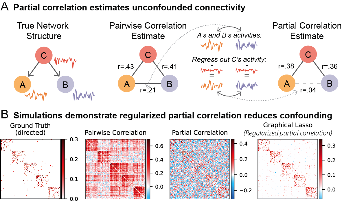
#Estimate glasso FC (a form of regularized partial correlation), using cross-validation to estimate the L1 regularization parameter
restFC_glassoFC=np.zeros((numnodes,numnodes,numsubjs))
scount=0
for subj in subjNums:
glassoFC_output=actflow.connectivity_estimation.graphicalLassoCV(restdata[:,:,scount])
restFC_glassoFC[:,:,scount]=glassoFC_output[0]
scount += 1
ADMM terminated after 152 iterations with status: optimal.
ADMM terminated after 140 iterations with status: optimal.
ADMM terminated after 147 iterations with status: optimal.
ADMM terminated after 149 iterations with status: optimal.
ADMM terminated after 143 iterations with status: optimal.
ADMM terminated after 147 iterations with status: optimal.
...
ADMM terminated after 14 iterations with status: optimal.
ADMM terminated after 11 iterations with status: optimal.
ADMM terminated after 26 iterations with status: optimal.
ADMM terminated after 14 iterations with status: optimal.
ADMM terminated after 104 iterations with status: optimal.
CPU times: user 2d 20h 1min 56s, sys: 49min 40s, total: 2d 20h 51min 36s
Wall time: 3h 33min 31s
#Visualize FC matrix
print('Group-average FC matrix')
fcmat_glasso=np.mean(restFC_glassoFC[netorder,:,:][:,netorder,:],axis=2)
fig=actflow.tools.addNetColors_Seaborn(fcmat_glasso)
Group-average FC matrix

#Visualize single-subject FC matrix
#fcmat_glasso=np.mean(restFC_glassoFC[netorder,:,:][:,netorder,:],axis=2)
print('Single-subject FC matrix')
fcmat_glasso_1subj=restFC_glassoFC[netorder,:,29][:,netorder]
fig=actflow.tools.addNetColors_Seaborn(fcmat_glasso_1subj)
Single-subject FC matrix

#Stats on FC matrices
FCdensities=np.zeros(numsubjs)
scount=0
for subj in subjNums:
    numNodes=np.shape(restFC_glassoFC)[0]
    FCdensities[scount]=np.sum(np.abs(restFC_glassoFC[:,:,scount])>0)/(numNodes*(numNodes-1))*100
    scount += 1

print('FC densities (100 X total # of non-zero connections / total possible connections):')
print('Mean:',np.mean(FCdensities),'%')
print('Stdev:',np.std(FCdensities),'%')
print('Range:',np.min(FCdensities),'% to',np.max(FCdensities),'%')
FC densities (100 X total # of non-zero connections / total possible connections):
Mean: 32.074331992159294 %
Stdev: 3.282696206876493 %
Range: 18.036211699164344 % to 38.16465490560198 %
#Run activity flow mapping with glasso (a form of regularized partial correlation)
print("==Activity flow mapping results, glasso-based resting-state FC, 24 task conditions==")
actflowOutput_restFCglassoFC_bycond = actflow.actflowcomp.actflowtest(activations_bycond, restFC_glassoFC)
==Activity flow mapping results, glasso-based resting-state FC, 24 task conditions==
===Comparing prediction accuracies between models (similarity between predicted and actual brain activation patterns)===

==Comparisons between predicted and actual activation patterns, across all conditions and nodes:==
--Compare-then-average (calculating prediction accuracies before cross-subject averaging):
Each comparison based on 24 conditions across 360 nodes, p-values based on 30 subjects (cross-subject variance in comparisons)

Mean Pearson r = 0.84, t-value vs. 0: 74.41, p-value vs. 0: 1.1541737098311694e-34

Mean % variance explained (R^2 score, coeff. of determination) = 0.70

Mean MAE (mean absolute error) = 6.34

Note: Pearson r and Pearson r^2 are scale-invariant, while R^2 and MAE are not. R^2 units: percentage of the to-be-predicted data's unscaled variance, ranging from negative infinity (because prediction errors can be arbitrarily large) to positive 1. See https://scikit-learn.org/stable/modules/generated/sklearn.metrics.r2_score.html for more info.
#Visualize predicted and actual activation patterns

plt.figure(figsize=[7,5])
ax = sns.heatmap(np.mean(actflowOutput_restFCglassoFC_bycond['actPredVector_bytask_bysubj'],axis=2)[netorder,:],center=0,cmap='seismic',cbar=True,yticklabels=100,xticklabels=taskConditions)
ax.figure.suptitle('Predicted activations, Glasso FC actflow')
ax.set(ylabel='Regions')

plt.figure(figsize=[7,5])
ax = sns.heatmap(np.mean(activations_bycond,axis=2)[netorder,:],center=0,cmap='seismic',cbar=True,yticklabels=100,xticklabels=taskConditions)
ax.figure.suptitle('Actual activations (24 conditions)')
ax.set(ylabel='Regions')
[Text(54.75, 0.5, 'Regions')]

#Plotting brain surface images in-line, FC-based predictions

condNum=12 #condition 9 = relational reasoning

#RestFC predicted
inputdata=np.mean(actflowOutput_restFCglassoFC_bycond['actPredVector_bytask_bysubj'],axis=2)[:,condNum]
print('Min value: ', np.min(inputdata))
print('Max value: ', np.max(inputdata))
#flip hemispheres, since CAB-NP is ordered left-to-right, while wbplot uses right-to-left
inputdata_flipped=np.zeros(np.shape(inputdata))
inputdata_flipped[0:180]=inputdata[180:360]
inputdata_flipped[180:360]=inputdata[0:180]
file_out="out.png"
#Set to all reds if no negative values
if min(inputdata) >= 0:
    colormap='Reds'
else:
    colormap='seismic'
pscalar(
        file_out=file_out,
        pscalars=inputdata_flipped,
        cmap=colormap,
        transparent=True)
img = mpimg.imread(file_out)
plt.figure()
plt.axis('off')
plt.title('Glasso rest FC actflow predictions (relational reasoning)')
plt.imshow(img)

#Actual activity
inputdata=np.mean(activations_bycond,axis=2)[:,condNum]
print('Min value: ', np.min(inputdata))
print('Max value: ', np.max(inputdata))
#flip hemispheres, since CAB-NP is ordered left-to-right, while wbplot uses right-to-left
inputdata_flipped=np.zeros(np.shape(inputdata))
inputdata_flipped[0:180]=inputdata[180:360]
inputdata_flipped[180:360]=inputdata[0:180]
file_out="out.png"
#Set to all reds if no negative values
if min(inputdata) >= 0:
    colormap='Reds'
else:
    colormap='seismic'
pscalar(
        file_out=file_out,
        pscalars=inputdata_flipped,
        cmap=colormap,
        transparent=True)
img = mpimg.imread(file_out)
plt.figure()
plt.axis('off')
plt.title('Actual activations (relational reasoning)')
plt.imshow(img)
pixdim[1,2,3] should be non-zero; setting 0 dims to 1
Min value:  -14.53952167876293
Max value:  30.413919582122137
Info: Time to read /tmp/HumanCorticalParcellations/S1200.L.flat.32k_fs_LR.surf.gii was 0.045721 seconds.


Info: Time to read /tmp/HumanCorticalParcellations/S1200.L.inflated_MSMAll.32k_fs_LR.surf.gii was 0.018488 seconds.


Info: Time to read /tmp/HumanCorticalParcellations/S1200.L.midthickness_MSMAll.32k_fs_LR.surf.gii was 0.028657 seconds.


Info: Time to read /tmp/HumanCorticalParcellations/S1200.L.very_inflated_MSMAll.32k_fs_LR.surf.gii was 0.017414 seconds.


Info: Time to read /tmp/HumanCorticalParcellations/S1200.R.flat.32k_fs_LR.surf.gii was 0.044146 seconds.


Info: Time to read /tmp/HumanCorticalParcellations/S1200.R.inflated_MSMAll.32k_fs_LR.surf.gii was 0.018327 seconds.


Info: Time to read /tmp/HumanCorticalParcellations/S1200.R.midthickness_MSMAll.32k_fs_LR.surf.gii was 0.028881 seconds.


Info: Time to read /tmp/HumanCorticalParcellations/S1200.R.very_inflated_MSMAll.32k_fs_LR.surf.gii was 0.017195 seconds.


Info: Time to read /tmp/ImageParcellated.dlabel.nii was 0.046372 seconds.

pixdim[1,2,3] should be non-zero; setting 0 dims to 1
Min value:  -20.209393092277782
Max value:  33.18593086232514
Info: Time to read /tmp/HumanCorticalParcellations/S1200.L.flat.32k_fs_LR.surf.gii was 0.045835 seconds.


Info: Time to read /tmp/HumanCorticalParcellations/S1200.L.inflated_MSMAll.32k_fs_LR.surf.gii was 0.018605 seconds.


Info: Time to read /tmp/HumanCorticalParcellations/S1200.L.midthickness_MSMAll.32k_fs_LR.surf.gii was 0.028713 seconds.


Info: Time to read /tmp/HumanCorticalParcellations/S1200.L.very_inflated_MSMAll.32k_fs_LR.surf.gii was 0.017382 seconds.


Info: Time to read /tmp/HumanCorticalParcellations/S1200.R.flat.32k_fs_LR.surf.gii was 0.044265 seconds.


Info: Time to read /tmp/HumanCorticalParcellations/S1200.R.inflated_MSMAll.32k_fs_LR.surf.gii was 0.018375 seconds.


Info: Time to read /tmp/HumanCorticalParcellations/S1200.R.midthickness_MSMAll.32k_fs_LR.surf.gii was 0.028553 seconds.


Info: Time to read /tmp/HumanCorticalParcellations/S1200.R.very_inflated_MSMAll.32k_fs_LR.surf.gii was 0.017225 seconds.


Info: Time to read /tmp/ImageParcellated.dlabel.nii was 0.046641 seconds.
<matplotlib.image.AxesImage at 0x7ffaceec40a0>

%%time
#Run activity flow mapping with combinedFC
restFC_combFC=np.zeros((numnodes,numnodes,numsubjs))
scount=0
for subj in subjNums:
    restFC_combFC[:,:,scount]=actflow.connectivity_estimation.combinedFC(restdata[:,:,scount])
    scount += 1

print("==Activity flow mapping results, combinedFC-based resting-state FC, 24 task conditions==")
actflowOutput_restFCcombFC_bycond = actflow.actflowcomp.actflowtest(activations_bycond, restFC_combFC)
==Activity flow mapping results, combinedFC-based resting-state FC, 24 task conditions==
===Comparing prediction accuracies between models (similarity between predicted and actual brain activation patterns)===

==Comparisons between predicted and actual activation patterns, across all conditions and nodes:==
--Compare-then-average (calculating prediction accuracies before cross-subject averaging):
Each comparison based on 24 conditions across 360 nodes, p-values based on 30 subjects (cross-subject variance in comparisons)

Mean Pearson r = 0.70, t-value vs. 0: 72.53, p-value vs. 0: 2.4170841995108216e-34

Mean % variance explained (R^2 score, coeff. of determination) = 0.46

Mean MAE (mean absolute error) = 8.56

Note: Pearson r and Pearson r^2 are scale-invariant, while R^2 and MAE are not. R^2 units: percentage of the to-be-predicted data's unscaled variance, ranging from negative infinity (because prediction errors can be arbitrarily large) to positive 1. See https://scikit-learn.org/stable/modules/generated/sklearn.metrics.r2_score.html for more info.
CPU times: user 30.3 s, sys: 1.68 s, total: 31.9 s
Wall time: 16 s
%%time
#Run multiple-regression FC using only the combinedFC-validated connections
#This adjusts the weights to better optimize for prediction, rather than using abstract r-values
#(see Cole, Michael W, Takuya Ito, Danielle S Bassett, and Douglas H Schultz. (2016). “Activity Flow over Resting-State Networks Shapes Cognitive Task Activations.” Nature Neuroscience 19 (12): 1718–26. doi:10.1038/nn.4406.)
restFC_mregCombFC=np.zeros((numnodes,numnodes,numsubjs))
scount=0
for subj in subjNums:
    restFC_mregCombFC[:,:,scount]=actflow.connectivity_estimation.multregconn(restdata[:,:,scount],conn_mask=(restFC_combFC[:,:,scount]!=0))
    scount += 1

print("==Activity flow mapping results, combinedFC+multreg-based resting-state FC, 24 task conditions==")
actflowOutput_restFCcombFCmultreg_bycond = actflow.actflowcomp.actflowtest(activations_bycond, restFC_mregCombFC)
==Activity flow mapping results, combinedFC+multreg-based resting-state FC, 24 task conditions==
===Comparing prediction accuracies between models (similarity between predicted and actual brain activation patterns)===

==Comparisons between predicted and actual activation patterns, across all conditions and nodes:==
--Compare-then-average (calculating prediction accuracies before cross-subject averaging):
Each comparison based on 24 conditions across 360 nodes, p-values based on 30 subjects (cross-subject variance in comparisons)

Mean Pearson r = 0.81, t-value vs. 0: 64.44, p-value vs. 0: 7.308483937481038e-33

Mean % variance explained (R^2 score, coeff. of determination) = 0.65

Mean MAE (mean absolute error) = 6.83

Note: Pearson r and Pearson r^2 are scale-invariant, while R^2 and MAE are not. R^2 units: percentage of the to-be-predicted data's unscaled variance, ranging from negative infinity (because prediction errors can be arbitrarily large) to positive 1. See https://scikit-learn.org/stable/modules/generated/sklearn.metrics.r2_score.html for more info.
CPU times: user 37.8 s, sys: 246 ms, total: 38.1 s
Wall time: 19.1 s
#Visualize FC matrix
fcmat=np.mean(restFC_mregCombFC[netorder,:,:][:,netorder,:],axis=2)
fig=actflow.tools.addNetColors_Seaborn(fcmat)

#Visualize predicted and actual activation patterns

plt.figure(figsize=[7,5])
ax = sns.heatmap(np.mean(actflowOutput_restFCcombFCmultreg_bycond['actPredVector_bytask_bysubj'],axis=2)[netorder,:],center=0,cmap='seismic',cbar=True,yticklabels=100,xticklabels=taskConditions)
ax.figure.suptitle('Predicted activations, combinedFC actflow')
ax.set(ylabel='Regions')

plt.figure(figsize=[7,5])
ax = sns.heatmap(np.mean(activations_bycond,axis=2)[netorder,:],center=0,cmap='seismic',cbar=True,yticklabels=100,xticklabels=taskConditions)
ax.figure.suptitle('Actual activations (24 conditions)')
ax.set(ylabel='Regions')
[Text(40.5, 0.5, 'Regions')]


#Plotting brain surface images in-line, FC-based predictions

condNum=12 #condition 9 = relational reasoning

#RestFC predicted
inputdata=np.mean(actflowOutput_restFCcombFCmultreg_bycond['actPredVector_bytask_bysubj'],axis=2)[:,condNum]
print('Min value: ', np.min(inputdata))
print('Max value: ', np.max(inputdata))
#flip hemispheres, since CAB-NP is ordered left-to-right, while wbplot uses right-to-left
inputdata_flipped=np.zeros(np.shape(inputdata))
inputdata_flipped[0:180]=inputdata[180:360]
inputdata_flipped[180:360]=inputdata[0:180]
file_out="out.png"
#Set to all reds if no negative values
if min(inputdata) >= 0:
    colormap='Reds'
else:
    colormap='seismic'
pscalar(
        file_out=file_out,
        pscalars=inputdata_flipped,
        cmap=colormap,
        transparent=True)
img = mpimg.imread(file_out)
plt.figure()
plt.axis('off')
plt.title('CombinedFC restFC actflow predictions (relational reasoning)')
plt.imshow(img)

#Actual activity
inputdata=np.mean(activations_bycond,axis=2)[:,condNum]
print('Min value: ', np.min(inputdata))
print('Max value: ', np.max(inputdata))
#flip hemispheres, since CAB-NP is ordered left-to-right, while wbplot uses right-to-left
inputdata_flipped=np.zeros(np.shape(inputdata))
inputdata_flipped[0:180]=inputdata[180:360]
inputdata_flipped[180:360]=inputdata[0:180]
file_out="out.png"
#Set to all reds if no negative values
if min(inputdata) >= 0:
    colormap='Reds'
else:
    colormap='seismic'
pscalar(
        file_out=file_out,
        pscalars=inputdata_flipped,
        cmap=colormap,
        transparent=True)
img = mpimg.imread(file_out)
plt.figure()
plt.axis('off')
plt.title('Actual activations (relational reasoning)')
plt.imshow(img)
pixdim[1,2,3] should be non-zero; setting 0 dims to 1
Min value:  -12.605234785397633
Max value:  28.306067880714533
pixdim[1,2,3] should be non-zero; setting 0 dims to 1
Min value:  -20.209393092277782
Max value:  33.18593086232514
<matplotlib.image.AxesImage at 0x7fc6b12e3710>


%%time
#Run activity flow mapping with ten subjects (to reduce processing time)

#Calculate multiple-regression FC
restFC_mreg=np.zeros((numnodes,numnodes,numsubjs))
for scount in np.arange(numsubjs):
    restFC_mreg[:,:,scount]=actflow.connectivity_estimation.multregconn(restdata[:,:,scount])
CPU times: user 2h 48min 27s, sys: 7min 13s, total: 2h 55min 40s
Wall time: 9min 5s
print("==Activity flow mapping results, multiple-regression-based resting-state FC, 24 task conditions==")
actflowOutput_restFCMReg_bycond = actflow.actflowcomp.actflowtest(activations_bycond, restFC_mreg)
==Activity flow mapping results, multiple-regression-based resting-state FC, 24 task conditions==
===Comparing prediction accuracies between models (similarity between predicted and actual brain activation patterns)===

==Comparisons between predicted and actual activation patterns, across all conditions and nodes:==
--Compare-then-average (calculating prediction accuracies before cross-subject averaging):
Each comparison based on 24 conditions across 360 nodes, p-values based on 30 subjects (cross-subject variance in comparisons)

Mean Pearson r = 0.78, t-value vs. 0: 62.27, p-value vs. 0: 1.9635597302245892e-32

Mean % variance explained (R^2 score, coeff. of determination) = 0.57

Mean MAE (mean absolute error) = 7.54

Note: Pearson r and Pearson r^2 are scale-invariant, while R^2 and MAE are not. R^2 units: percentage of the to-be-predicted data's unscaled variance, ranging from negative infinity (because prediction errors can be arbitrarily large) to positive 1. See https://scikit-learn.org/stable/modules/generated/sklearn.metrics.r2_score.html for more info.
#Visualize multreg FC matrix
fcmat=np.mean(restFC_mreg[netorder,:,:][:,netorder,:],axis=2)
fig=actflow.tools.addNetColors_Seaborn(fcmat)

#Visualize predicted and actual activation patterns, with multiple-regression FC
plt.figure(figsize=[7,5])
ax = sns.heatmap(np.mean(actflowOutput_restFCMReg_bycond['actPredVector_bytask_bysubj'],axis=2)[netorder,:],center=0,cmap='seismic',cbar=True,cbar_kws={'label': 'Activation'},yticklabels=100,xticklabels=taskConditions)
ax.figure.suptitle('Predicted activations, multreg FC actflow')
ax.set(ylabel='Regions')

plt.figure(figsize=[7,5])
#Activation (z-score)
ax = sns.heatmap(np.mean(activations_bycond,axis=2)[netorder,:],center=0,cmap='seismic',cbar=True,cbar_kws={'label': 'Activation'},yticklabels=100,xticklabels=taskConditions)
ax.figure.suptitle('Actual activations (24 conditions)')
ax.set(ylabel='Regions')
[Text(39.5, 0.5, 'Regions')]


#Plotting brain surface images in-line, FC-based predictions

condNum=12 #condition 9 = relational reasoning

#RestFC predicted
inputdata=np.mean(actflowOutput_restFCMReg_bycond['actPredVector_bytask_bysubj'],axis=2)[:,condNum]
print('Min value: ', np.min(inputdata))
print('Max value: ', np.max(inputdata))
#flip hemispheres, since CAB-NP is ordered left-to-right, while wbplot uses right-to-left
inputdata_flipped=np.zeros(np.shape(inputdata))
inputdata_flipped[0:180]=inputdata[180:360]
inputdata_flipped[180:360]=inputdata[0:180]
file_out="out.png"
#Set to all reds if no negative values
if min(inputdata) >= 0:
    colormap='Reds'
else:
    colormap='seismic'
pscalar(
        file_out=file_out,
        pscalars=inputdata_flipped,
        cmap=colormap,
        transparent=True)
img = mpimg.imread(file_out)
plt.figure()
plt.axis('off')
plt.title('Multreg restFC actflow predictions (relational reasoning)')
plt.imshow(img)

#Actual activity
inputdata=np.mean(activations_bycond,axis=2)[:,condNum]
print('Min value: ', np.min(inputdata))
print('Max value: ', np.max(inputdata))
#flip hemispheres, since CAB-NP is ordered left-to-right, while wbplot uses right-to-left
inputdata_flipped=np.zeros(np.shape(inputdata))
inputdata_flipped[0:180]=inputdata[180:360]
inputdata_flipped[180:360]=inputdata[0:180]
file_out="out.png"
#Set to all reds if no negative values
if min(inputdata) >= 0:
    colormap='Reds'
else:
    colormap='seismic'
pscalar(
        file_out=file_out,
        pscalars=inputdata_flipped,
        cmap=colormap,
        transparent=True)
img = mpimg.imread(file_out)
plt.figure()
plt.axis('off')
plt.title('Actual activations (relational reasoning)')
plt.imshow(img)
pixdim[1,2,3] should be non-zero; setting 0 dims to 1
Min value:  -16.59970533540053
Max value:  26.27911656833697
Min value:  -20.209393092277782
Max value:  33.18593086232514
pixdim[1,2,3] should be non-zero; setting 0 dims to 1
<matplotlib.image.AxesImage at 0x7efe144381d0>


print("===Compare resting-state multregFC actflow predictions to resting-state corrFC actflow prediction, 10 subjects only===")
model_compare_RestMultRegFCVsRestCorrFC_Actflow = actflow.model_compare(target_actvect=actflowOutput_restFCCorr_bycond['actVect_actual_group'][:,:,0:10], model1_actvect=actflowOutput_restFCMReg_bycond['actPredVector_bytask_bysubj'], model2_actvect=actflowOutput_restFCCorr_bycond['actPredVector_bytask_bysubj'][:,:,0:10], full_report=False, print_report=True)
===Compare resting-state multregFC actflow predictions to resting-state corrFC actflow prediction, 10 subjects only===
===Comparing prediction accuracies between models (similarity between predicted and actual brain activation patterns)===

==Comparisons between predicted and actual activation patterns, across all conditions and nodes:==
--Compare-then-average (calculating prediction accuracies before cross-subject averaging):
Each comparison based on 24 conditions across 360 nodes, p-values based on 10 subjects (cross-subject variance in comparisons)

Model1 mean Pearson r=0.78
Model2 mean Pearson r=0.59
R-value difference = 0.20
Model1 vs. Model2 T-value: 12.81, p-value: 4.4133474737407104e-07

Model1 mean % predicted variance explained R^2=0.58
Model2 mean % predicted variance explained R^2=-595.00
R^2 difference = 595.57

Model1 mean MAE = 7.08
Model2 mean MAE = 277.10
Model1 vs. Model2 mean MAE difference = -270.02

Note: Pearson r and Pearson r^2 are scale-invariant, while R^2 and MAE are not. R^2 units: percentage of the to-be-predicted data's unscaled variance, ranging from negative infinity (because prediction errors can be arbitrarily large) to positive 1. See https://scikit-learn.org/stable/modules/generated/sklearn.metrics.r2_score.html for more info.
print("===Compare TASK CONDITIONS SEPARATE, resting-state multregFC actflow predictions to resting-state corrFC actflow prediction, 10 subjects only===")
model_compare_RestMultRegFCVsRestCorrFC_Actflow_nodewise = actflow.model_compare(target_actvect=actflowOutput_restFCCorr_bycond['actVect_actual_group'][:,:,0:10], model1_actvect=actflowOutput_restFCMReg_bycond['actPredVector_bytask_bysubj'], model2_actvect=actflowOutput_restFCCorr_bycond['actPredVector_bytask_bysubj'][:,:,0:10], comparison_type='nodewise_compthenavg', full_report=False, print_report=True)
===Compare TASK CONDITIONS SEPARATE, resting-state multregFC actflow predictions to resting-state corrFC actflow prediction, 10 subjects only===
===Comparing prediction accuracies between models (similarity between predicted and actual brain activation patterns)===

==Node-wise (spatial) correlations between predicted and actual activation patterns (calculated for each condition separetely):==
--Compare-then-average (calculating prediction accuracies before cross-subject averaging):
Each correlation based on N nodes: 360, p-values based on N subjects (cross-subject variance in correlations): 10
Model1 mean Pearson r=0.74
Model2 mean Pearson r=0.56
R-value difference = 0.18
Model1 vs. Model2 T-value: 21.83, p-value: 4.185118497632039e-09
By task condition:
Condition 1: Model 1 r=0.62, Model 2 r=0.52, Model 1 vs. 2 R-value difference =0.10, t-value Model1 vs. Model2: 6.48, p-value vs. 0: 0.00011350821684287335
Condition 2: Model 1 r=0.62, Model 2 r=0.49, Model 1 vs. 2 R-value difference =0.13, t-value Model1 vs. Model2: 4.50, p-value vs. 0: 0.0014834154061634732
Condition 3: Model 1 r=0.81, Model 2 r=0.66, Model 1 vs. 2 R-value difference =0.15, t-value Model1 vs. Model2: 10.75, p-value vs. 0: 1.9500887302004183e-06
Condition 4: Model 1 r=0.81, Model 2 r=0.65, Model 1 vs. 2 R-value difference =0.16, t-value Model1 vs. Model2: 11.69, p-value vs. 0: 9.63880144345734e-07
Condition 5: Model 1 r=0.66, Model 2 r=0.36, Model 1 vs. 2 R-value difference =0.30, t-value Model1 vs. Model2: 8.75, p-value vs. 0: 1.0719708060750169e-05
Condition 6: Model 1 r=0.66, Model 2 r=0.38, Model 1 vs. 2 R-value difference =0.29, t-value Model1 vs. Model2: 11.34, p-value vs. 0: 1.2404568347342055e-06
Condition 7: Model 1 r=0.77, Model 2 r=0.63, Model 1 vs. 2 R-value difference =0.14, t-value Model1 vs. Model2: 8.64, p-value vs. 0: 1.191965484960132e-05
Condition 8: Model 1 r=0.65, Model 2 r=0.45, Model 1 vs. 2 R-value difference =0.20, t-value Model1 vs. Model2: 4.55, p-value vs. 0: 0.0013876834268410519
Condition 9: Model 1 r=0.60, Model 2 r=0.50, Model 1 vs. 2 R-value difference =0.10, t-value Model1 vs. Model2: 2.47, p-value vs. 0: 0.03528215084400667
Condition 10: Model 1 r=0.64, Model 2 r=0.48, Model 1 vs. 2 R-value difference =0.16, t-value Model1 vs. Model2: 7.03, p-value vs. 0: 6.097046675792787e-05
Condition 11: Model 1 r=0.59, Model 2 r=0.42, Model 1 vs. 2 R-value difference =0.16, t-value Model1 vs. Model2: 4.89, p-value vs. 0: 0.0008631876315222374
Condition 12: Model 1 r=0.64, Model 2 r=0.42, Model 1 vs. 2 R-value difference =0.22, t-value Model1 vs. Model2: 4.53, p-value vs. 0: 0.0014309469747718026
Condition 13: Model 1 r=0.81, Model 2 r=0.66, Model 1 vs. 2 R-value difference =0.15, t-value Model1 vs. Model2: 7.90, p-value vs. 0: 2.438376969888114e-05
Condition 14: Model 1 r=0.82, Model 2 r=0.69, Model 1 vs. 2 R-value difference =0.13, t-value Model1 vs. Model2: 7.65, p-value vs. 0: 3.144822647925268e-05
Condition 15: Model 1 r=0.78, Model 2 r=0.59, Model 1 vs. 2 R-value difference =0.19, t-value Model1 vs. Model2: 7.50, p-value vs. 0: 3.702467116064869e-05
Condition 16: Model 1 r=0.80, Model 2 r=0.68, Model 1 vs. 2 R-value difference =0.12, t-value Model1 vs. Model2: 7.56, p-value vs. 0: 3.469297986943825e-05
Condition 17: Model 1 r=0.77, Model 2 r=0.60, Model 1 vs. 2 R-value difference =0.17, t-value Model1 vs. Model2: 6.25, p-value vs. 0: 0.00015033734222864376
Condition 18: Model 1 r=0.72, Model 2 r=0.55, Model 1 vs. 2 R-value difference =0.18, t-value Model1 vs. Model2: 8.67, p-value vs. 0: 1.1543967905031033e-05
Condition 19: Model 1 r=0.81, Model 2 r=0.59, Model 1 vs. 2 R-value difference =0.22, t-value Model1 vs. Model2: 7.39, p-value vs. 0: 4.135200027225793e-05
Condition 20: Model 1 r=0.82, Model 2 r=0.64, Model 1 vs. 2 R-value difference =0.18, t-value Model1 vs. Model2: 8.26, p-value vs. 0: 1.7089544872121718e-05
Condition 21: Model 1 r=0.80, Model 2 r=0.63, Model 1 vs. 2 R-value difference =0.17, t-value Model1 vs. Model2: 13.22, p-value vs. 0: 3.3669498324749096e-07
Condition 22: Model 1 r=0.75, Model 2 r=0.56, Model 1 vs. 2 R-value difference =0.19, t-value Model1 vs. Model2: 10.80, p-value vs. 0: 1.8738523022025353e-06
Condition 23: Model 1 r=0.80, Model 2 r=0.55, Model 1 vs. 2 R-value difference =0.25, t-value Model1 vs. Model2: 10.46, p-value vs. 0: 2.464690686607065e-06
Condition 24: Model 1 r=0.81, Model 2 r=0.61, Model 1 vs. 2 R-value difference =0.20, t-value Model1 vs. Model2: 9.13, p-value vs. 0: 7.5608701761735165e-06
ax = sns.scatterplot(np.arange(24),np.mean(model_compare_RestMultRegFCVsRestCorrFC_Actflow_nodewise['corr_nodewise_compthenavg_bycond'],axis=1), s=100)
ax.figure.suptitle('Pred.-to-actual accuracies for each condition (whole-brain activity patterns)')
ax.set(ylabel='Pearson correlation')
ax.set(xlabel='Task condition')
[Text(0.5, 0, 'Task condition')]

ax = sns.scatterplot(np.arange(24),np.mean(model_compare_RestMultRegFCVsRestCorrFC_Actflow_nodewise['R2_nodewise_compthenavg_bycond'],axis=1), s=100)
ax.figure.suptitle('Pred.-to-actual accuracies for each condition (whole-brain activity patterns)')
ax.set(ylabel='R^2 (unscaled % variance)')
ax.set(xlabel='Task condition')
[Text(0.5, 0, 'Task condition')]

print("===Compare REGIONS SEPARATE (24-condition response profiles), resting-state multregFC actflow predictions to resting-state corrFC actflow prediction, 10 subjects only===")
model_compare_RestMultRegFCVsRestCorrFC_Actflow_condwise = actflow.model_compare(target_actvect=actflowOutput_restFCCorr_bycond['actVect_actual_group'][:,:,0:10], model1_actvect=actflowOutput_restFCMReg_bycond['actPredVector_bytask_bysubj'], model2_actvect=actflowOutput_restFCCorr_bycond['actPredVector_bytask_bysubj'][:,:,0:10], comparison_type='conditionwise_compthenavg', full_report=False, print_report=True)
===Compare REGIONS SEPARATE (24-condition response profiles), resting-state multregFC actflow predictions to resting-state corrFC actflow prediction, 10 subjects only===
===Comparing prediction accuracies between models (similarity between predicted and actual brain activation patterns)===

==Condition-wise comparisons between predicted and actual activation patterns (calculated for each node separetely):==
--Compare-then-average (calculating prediction accuracies before cross-subject averaging):
Each correlation based on N conditions: 24, p-values based on N subjects (cross-subject variance in correlations): 10

Model1 mean Pearson r=0.81
Model2 mean Pearson r=0.62
R-value difference = 0.19
Model1 vs. Model2 T-value: 12.46, p-value: 5.572065132326254e-07

Model1 mean % predicted variance explained R^2=0.09
Model2 mean % predicted variance explained R^2=-1450.42
R^2 difference = 1450.51

Model1 mean MAE = 7.08
Model2 mean MAE = 277.10
Model1 vs. Model2 mean MAE difference = -270.02

Note: Pearson r and Pearson r^2 are scale-invariant, while R^2 and MAE are not. R^2 units: percentage of the to-be-predicted data's unscaled variance, ranging from negative infinity (because prediction errors can be arbitrarily large) to positive 1. See https://scikit-learn.org/stable/modules/generated/sklearn.metrics.r2_score.html for more info.
plt.figure(figsize=[7,5])
ax = sns.scatterplot(np.arange(360),np.mean(model_compare_RestMultRegFCVsRestCorrFC_Actflow_condwise['corr_conditionwise_compthenavg_bynode'],axis=1), s=50)
ax.figure.suptitle('Pred.-to-actual accuracies for each region (24-condition response profiles)')
ax.set(ylabel='Pearson correlation')
ax.set(xlabel='Region')
[Text(0.5, 0, 'Region')]

plt.figure(figsize=[7,5])
ax = sns.scatterplot(np.arange(360),np.mean(model_compare_RestMultRegFCVsRestCorrFC_Actflow_condwise['R2_conditionwise_compthenavg_bynode'],axis=1), s=50)
ax.figure.suptitle('Pred.-to-actual accuracies for each region (24-condition response profiles)')
ax.set(ylabel='R^2 (unscaled % variance)')
ax.set(xlabel='Region')
[Text(0.5, 0, 'Region')]

It is known that fMRI has some inherent spatial smoothness that blurs data spatially due to local vasculature. This smoothness is thought to extend somewhere between 2 mm and 5 mm (Malonek and Grinvald 1996; Logothetis and Wandell 2004). In theory this could result in some circularity to the actflow predictions (e.g., the target region's activity blurs into a source region's activity). The code below demonstrates an approach to remove any region within 10 mm of each to-be-predicted target region, removing any potential circularity due to vascular spatial smoothness. Note that there was only a small reduction in prediction accuracy in the results below (likely due to having fewer predictors), suggesting spatial smoothness results in minor (if any) prediction circularity.
#Load dictionary listing which parcels to exclude for each target
networkdefdir = pkg_resources.resource_filename('ActflowToolbox', 'network_definitions/')
inputfilename = networkdefdir+'parcels_to_remove_indices_cortexonly_data.h5'
h5f = h5py.File(inputfilename,'r')
parcels_to_remove={}
for parcelInt in range(numnodes):
    outname1 = 'parcels_to_remove_indices'+'/'+str(parcelInt)
    parcels_to_remove[parcelInt] = h5f[outname1][:].copy()
h5f.close()
%%time

#Calculate multiple-regression FC, excluding parcels within 10 mm of each target parcel
restFC_mreg_parcelnoncirc=np.zeros((numnodes,numnodes,numsubjs))
for scount in np.arange(numsubjs):
    restFC_mreg_parcelnoncirc[:,:,scount]=actflow.connectivity_estimation.multregconn(restdata[:,:,scount], parcelstoexclude_bytarget=parcels_to_remove)
CPU times: user 2h 14min 31s, sys: 5min 15s, total: 2h 19min 47s
Wall time: 6min 59s
print("==Activity flow mapping results, multiple-regression-based resting-state FC (parcel non-circular), 24 task conditions==")
actflowOutput_restFCMReg_parcelnoncirc_bycond = actflow.actflowcomp.actflowtest(activations_bycond, restFC_mreg_parcelnoncirc)
==Activity flow mapping results, multiple-regression-based resting-state FC (parcel non-circular), 24 task conditions==
===Comparing prediction accuracies between models (similarity between predicted and actual brain activation patterns)===

==Comparisons between predicted and actual activation patterns, across all conditions and nodes:==
--Compare-then-average (calculating prediction accuracies before cross-subject averaging):
Each comparison based on 24 conditions across 360 nodes, p-values based on 30 subjects (cross-subject variance in comparisons)

Mean Pearson r = 0.73, t-value vs. 0: 54.55, p-value vs. 0: 8.804966610436179e-31

Mean % variance explained (R^2 score, coeff. of determination) = 0.50

Mean MAE (mean absolute error) = 8.19

Note: Pearson r and Pearson r^2 are scale-invariant, while R^2 and MAE are not. R^2 units: percentage of the to-be-predicted data's unscaled variance, ranging from negative infinity (because prediction errors can be arbitrarily large) to positive 1. See https://scikit-learn.org/stable/modules/generated/sklearn.metrics.r2_score.html for more info.
#Visualize multreg noncircular FC matrix
fcmat=np.mean(restFC_mreg_parcelnoncirc[netorder,:,:][:,netorder,:],axis=2)
fig=actflow.tools.addNetColors_Seaborn(fcmat)
